This post contains our crib notes on the basics of decision trees and forests. We first discuss the construction of individual trees, and then introduce random and boosted forests. We also discuss efficient implementations of greedy tree construction algorithms, showing that a single tree can be constructed in \(O(k \times n \log n)\) time, given \(n\) training examples having \(k\) features each. We provide exercises on interesting related points and an appendix containing relevant python/sk-learn function calls.
Introduction
Decision trees constitute a class of simple functions that are frequently used for carrying out regression and classification. They are constructed by hierarchically splitting a feature space into disjoint regions, where each split divides into two one of the already existing regions. In most common implementations, the splits are always taken along one of the feature axes, which causes the regions to be rectangular in shape. An example is shown in Fig. 1 below. In this example, a two-dimensional feature space is first split by a tree on \(f_1\) — one of the two features characterizing the space — at value \(s_a\). This separates the space into two sets, that where \(f_1 < s_a\) and that where \(f_1 \geq s_a\). Next, the tree further splits the first of these sets on feature \(f_2\) at value \(s_b\). With these combined splits, the tree partitions the space into three disjoint regions, labeled \(R_1, R_2,\) and \(R_3\), where, e.g., \(R_1 = \{ \textbf{f} \vert f_1 < s_a, f_2 < s_b \}\).
Once a decision tree is constructed, it can be used for making predictions on unlabeled feature vectors — i.e., points in feature space not included in our training set. This is done by first deciding which of the regions a new feature vector belongs to, and then returning as its hypothesis label an average over the training example labels within that region: The mean of the region’s training labels is returned for regression problems and the mode for classification problems. For instance, the tree in Fig. 1 would return an average of the five training examples in \(R_1\) (represented by red dots) when asked to make a hypothesis for any and all other points in that region.
The art and science of tree construction is in deciding how many splits should be taken and where those splits should take place. The goal is to find a tree that provides a reasonable, piece-wise constant approximation to the underlying distribution or function that has generated the training data provided. This can be attempted through choosing a tree that breaks space up into regions such that the examples in any given region have identical — or at least similar — labels. We discuss some common approaches to finding such trees in the next section.
Individual trees have the important benefit of being easy to interpret and visualize, but they are often not as accurate as other common machine learning algorithms. However, individual trees can be used as simple building blocks with which to construct more complex, competitive models. In the third section of this note, we discuss three very popular constructions of this sort: bagging, random forests (a variant on bagging), and boosting. We then discuss the runtime complexity of tree/forest construction and conclude with a summary, exercises, and an appendix containing example python code.
Constructing individual decision trees
Regression
Regression tree construction typically proceeds by attempting to minimize a squared error cost function: Given a training set \(T \equiv \{t_j = (\textbf{f}_j, y_j) \}\) of feature vectors and corresponding real-valued labels, this is given by
where \(\overline{y}_{R_i}\) is the mean training label in region \(R_i\). This mean training label is the hypothesis returned by the tree for all points in \(R_i\), including its training examples. Therefore, (\ref{treecost}) is a measure of the accuracy of the tree as applied to the training set.
Unfortunately, actually minimizing (\ref{treecost}) over any large subset of trees can be a numerically challenging task. This is true whenever you have a large number of features or training examples. Consequently, different approximate methods are generally taken to find good candidate trees. Two typical methods follow:
- Greedy algorithm: The tree is constructed recursively, one branching step at a time. At each step, one takes the split that will most significantly reduce the cost function \(J\), relative to its current value. In this way, after \(k-1\) splits, a tree with \(k\) regions (leaves) is obtained — Fig. 2 provides an illustration of this process. The algorithm terminates whenever some specified stopping criterion is satisfied, examples of which are given below.
- Randomized algorithm: Randomized tree-search protocols can sometimes find global minima inaccessible to the gradient-descent-like greedy algorithm. These randomized protocols also proceed recursively. However, at each step, some randomization is introduced by hand. For example, one common approach is to select \(r\) candidate splits through random sampling at each branching point. The candidate split that most significantly reduces \(J\) is selected, and the process repeats. The benefit of this approach is that it can sometimes find paths that appear suboptimal in their first few steps, but are ultimately favorable.
Classification
In classification problems, the training labels take on a discrete set of values, often having no numerical significance. This means that a squared-error cost function, like that in (\ref{treecost}) — cannot be directly applied as a useful accuracy score for guiding classification tree construction. Instead, three other cost functions are often considered, each providing a different measure of the class purity of the different regions — that is, they attempt to measure whether or not a given region consists of training examples that are mostly of the same class. These three measures are the error rate (\(E\)), the Gini index (\(G\)), and the cross-entropy (\(CE\)): If we write \(N_i\) for the number of training examples in region \(R_i\), and \(p_{i,j}\) for the fraction of these that have class label \(j\), then these three cost functions are given by
Each of the summands here are plotted in Fig. 3 for the special case of binary classification (two labels only). Each is unfavorably maximized at the most mixed state, where \(p_1 = 0.5\), and minimized in the pure states, where \(p_1 = 0,1\).
Although \(E\) is perhaps the most intuitive of the three measures above (it’s simply the number of training examples misclassified by the tree — this follows from the fact that the tree returns as hypothesis the mode in each region) the latter two have the benefit of being characterized by negative curvature as a function of the \(p_{i,j}\). This property tends to enhance the favorability of splits that generate region pairs where at least one is highly pure. At times, this can simultaneously result in the other region of the pair ending up relatively impure — see Exercise 1 for details. Such moves are often ultimately beneficial, since any highly impure node that results can always be broken up in later splits anyways. The plot in Fig. 3 shows that the cross-entropy has the larger curvature of the two, and so should more highly favor such splits, at least in the binary classification case. Another nice feature of the Gini and cross-entropy functions is that — in contrast to the error rate — they are both smooth functions of the \(p_{i,j}\), which facilitates numerical optimization. For these reasons, one of these two functions is typically used to guide tree construction, even if \(E\) is the quantity one would actually like to minimize. Tree construction proceeds as in the regression case, typically by a greedy or randomized construction, each step taken so as to minimize (\ref{gini}) or (\ref{crossentropy}), whichever is chosen.
Bias-variance trade-off and stopping conditions
Decision trees that are allowed to split indefinitely will have low bias but will over-fit their training data. Placing different stopping criteria on a tree’s growth can ameliorate this latter effect. Two typical conditions often used for this purpose are given by a) placing an upper bound on the number of levels permitted in the tree, or b) requiring that each region (tree leaf) retains at least some minimum number of training examples. To optimize over such constraints, one can apply cross-validation.
Bagging, random forests, and boosting
Another approach to alleviating the high-variance, over-fitting issue associated with decision trees is to average over many of them. This approach is motivated by the observation that the sum of \(N\) independent random variables — each with variance \(\sigma^2\) — has a relatively reduced variance, \(\sigma^2/N\). Two common methods for carrying out summations of this sort are discussed below.
Bagging and random forests
Bootstrap aggregation, or “bagging”, provides one common method for constructing ensemble tree models. In this approach, one samples with replacement to obtain \(k\) separate bootstrapped training sets from the original training data. To obtain a bootstrapped subsample of a data set of size \(N\), one draws randomly from the set \(N\) times with replacement. Because one samples with replacement, each bootstrapped set can contain multiple copies of some examples. The average number of unique examples in a given bootstrap is simply \(N\) times the probability that any individual example makes it into the training set. This is
where the latter forms are accurate in the large \(N\) limit. Once the bootstrapped data sets are constructed, an individual decision tree is fit to each, and an average or majority rule vote over the full set is used to provide the final prediction.
One nice thing about bagging methods, in general, is that one can train on the entire set of available labeled training data and still obtain an estimate of the generalization error. Such estimates are obtained by considering the error on each point in the training set, in each case averaging only over those trees that did not train on the point in question. The resulting estimate, called the out-of-bag error, typically provides a slight overestimate to the generalization error. This is because accuracy generally improves with growing ensemble size, and the full ensemble is usually about three times larger than the sub-ensemble used to vote on any particular training example in the out-of-bag error analysis.
Random forests provide a popular variation on the bagging method. The individual decision trees making up a random forest are, again, each fit to an independent, bootstrapped subsample of the training data. However, at each step in their recursive construction process, these trees are restricted in that they are only allowed to split on \(r\) randomly selected candidate feature directions; a new set of \(r\) directions is chosen at random for each step in the tree construction. These restrictions serve to effect a greater degree of independence in the set of trees averaged over in a random forest, which in turn serves to reduce the ensemble’s variance — see Exercise 5 for related analysis. In general, the value of \(r\) should be optimized through cross-validation.
Boosting
The final method we’ll discuss is boosting, which again consists of a set of individual trees that collectively determine the ultimate prediction returned by the model. However, in the boosting scenario, one fits each of the trees to the full data set, rather than to a small sample. Because they are fit to the full data set, these trees are usually restricted to being only two or three levels deep, so as to avoid over-fitting. Further, the individual trees in a boosted forest are constructed sequentially. For instance, in regression, the process typically works as follows: In the first step, a tree is fit to the full, original training set \(T = \{t_i = (\textbf{f}_i, y_i)\}\). Next, a second tree is constructed on the same training feature vectors, but with the original labels replaced by residuals. These residuals are obtained by subtracting out a scaled version of the predictions \(\hat{y}^1\) returned by the first tree,
Here, \(\alpha\) is the scaling factor, or learning rate — choosing its value small results in a gradual learning process, which often leads to very good predictions. Once the second tree is constructed, a third tree is fit to the new residuals, obtained by subtracting out the scaled hypothesis of the second tree, \(y_i^{(2)} \equiv y_i^{(1)} - \alpha \hat{y}_i^2\). The process repeats until \(m\) trees are constructed, with their \(\alpha\)-scaled hypotheses summing to a good estimate to the underlying function.
Boosted classification tree ensembles are constructed in a fashion similar to that above. However, in contrast to the regression scenario, the same, original training labels are used to fit each new tree in the ensemble (as opposed to an evolving residual). To bring about a similar, gradual learning process, boosted classification ensembles instead sample from the training set with weights that are sample-dependent and that change over time: When constructing a new tree for the ensemble, one more heavily weights those examples that have been poorly fit in prior iterations. AdaBoost is a popular algorithm for carrying out boosted classification. This and other generalizations are covered in the text Elements of Statistical Learning.
Implementation runtime complexity
Before concluding, we take here a moment to consider the runtime complexity of tree construction. This exercise gives one a sense of how tree algorithms are constructed in practice. We begin by considering the greedy construction of a single classification tree. The extension to regression trees is straightforward.
Individual decision trees
Consider the problem of greedily training a single classification tree on a set of \(n\) training examples having \(k\) features. In order to construct our tree, we take as a first step the sorting of the \(n\) training vectors along each of the \(k\) directions, which will facilitate later optimal split searches. Recall that optimized algorithms, e.g. merge-sort, require \(O(n \log n)\) time to sort along any one feature direction, so sorting along all \(k\) will require \(O(k \times n \log n)\) time. After this pre-sort step is complete, we must seek the currently optimal split, carry it out, and then iterate. We will show that — with care — the full iterative process can also be carried out in \(O(k \times n \log n)\) time.
Focus on an intermediate moment in the construction process where one particular node has just been split, resulting in two new regions, \(R_1\) and \(R_2\) containing \(n_{R_1}\) and \(n_{R_2}\) training examples, respectively. We can assume that we have already calculated and stored the optimal split for every other region in the tree during prior iterations. Therefore, to determine which region contains the next optimal split, the only new searches we need to carry out are within regions \(R_1\) and \(R_2\). Focus on \(R_1\) and suppose that we have been passed down the following information characterizing it: the number of training examples of each class that it contains, its total number of training examples \(n_{R_1}\), its cost function value \(J\) (cross entropy, say), and for each of the \(k\) feature directions, a separate list of the region’s examples, sorted along that direction. To find the optimal split, we must consider all \(k \times (n_{R_1}-1)\) possible cuts of this region [Aside: We must check all possible cuts because the cost function can have many local minima. The precludes the use of gradient-descent-like algorithms to find the optimal split.], evaluating the cost function reduction for each.
The left side of Fig. 4 illustrates one method for efficiently carrying out these test cuts: For each feature direction, we proceed sequentially through that direction’s ordered list, considering one cut at a time. In the first cut, we take only one example in the left sub-region induced, and all others on the right. In the second cut, we have the first two examples in the left sub-region, etc. Proceeding in this way, it turns out that the cost function of each new candidate split considered can always be evaluated in \(O(1)\) time. This is because we start with knowledge of the cost function \(J\) before any cut is taken, and the cost functions we consider here can each be updated in \(O(1)\) time whenever only a single example is either added to or removed from a given region — see exercises 3 and 4 for details. Using this approach, we can therefore try all possible cuts of region \(R_1\) in \(O(k \times n_{R_1})\) time.
The above analysis gives the time needed to search for the optimal split within \(R_1\), and a similar form holds for \(R_2\). Once these are determined, we can quickly select the current, globally-optimal split [Aside: Using a heap data structure, the global minimum can be obtained in at most \(O(\log n)\) time. Summing this effort over all nodes of the tree will lead to roughly \(O(n \log n)\) evaluations.]. Carrying out this split entails partitioning the region selected into two and passing the necessary information down to each. We leave as an exercise the fact that the passing of needed information — ordered lists, etc. — can be carried out in \(O(k \times n_s)\) time, with \(n_s\) the size of the parent region being split. The total tree construction time can now be obtained by summing up each node’s search and split work, which both require \(O(k \times n_s\)) computations. Assuming a roughly balanced tree having about \(\log n\) layers — see right side of Fig. 4 — we obtain \(O(k \times n \log n)\), the runtime scaling advertised.
In summary, we see that achieving \(O(k \times n \log n)\) scaling requires a) a pre-sort, b) a data structure for storing certain important facts about each region, including its optimal split, once determined, and also pointers to its parent and children, c) an efficient method for passing relevant information down to daughter regions during a split instance, d) a heap to enable quick selection of the currently optimal split, and e) a cost function that can be updated efficiently under single training example insertions or removals.
Forests, parallelization
If a forest of \(N\) trees is to be constructed, each will require \(O(k \times n \log n)\) time to construct. Recall, however, that the trees of a bagged forest can be constructed independently of one another. This allows for bagged forest constructions to take advantage of parallelization, facilitating their application in the large \(N\) limit. In contrast, the trees of a boosted forest are constructed in sequence and so cannot be parallelized in a similar manner. However, note that optimal split searches along different feature directions can always be run in parallel. This can speed up individual tree construction times in either case.
Discussion
In this note, we’ve quickly reviewed the basics of tree-based models and their constructions. Looking back over what we have learned, we can now consider some of the reasons why tree-based methods are so popular among practitioners. First — and very importantly — individual trees are often useful for gaining insight into the geometry of datasets in high dimensions. This is because tree structures can be visualized using simple diagrams, like that in Fig. 1. In contrast, most other machine learning algorithm outputs cannot be easily visualized — consider, e.g., support-vector machines, which return hyper-plane decision boundaries. A related point is that tree-based approaches are able to automatically fit non-linear decision boundaries. In contrast, linear algorithms can only fit such boundaries if appropriate non-linear feature combinations are constructed. This requires that one first identify these appropriate feature combinations, which can be a challenging task for feature spaces that cannot be directly visualized. Three additional positive qualities of decision trees are given by a) the fact that they are insensitive to feature scale, which reduces the need for related data preprocessing, b) the fact that they can make use of data missing certain feature values, and c) that they are relatively robust against outliers and noisy-labeling issues.
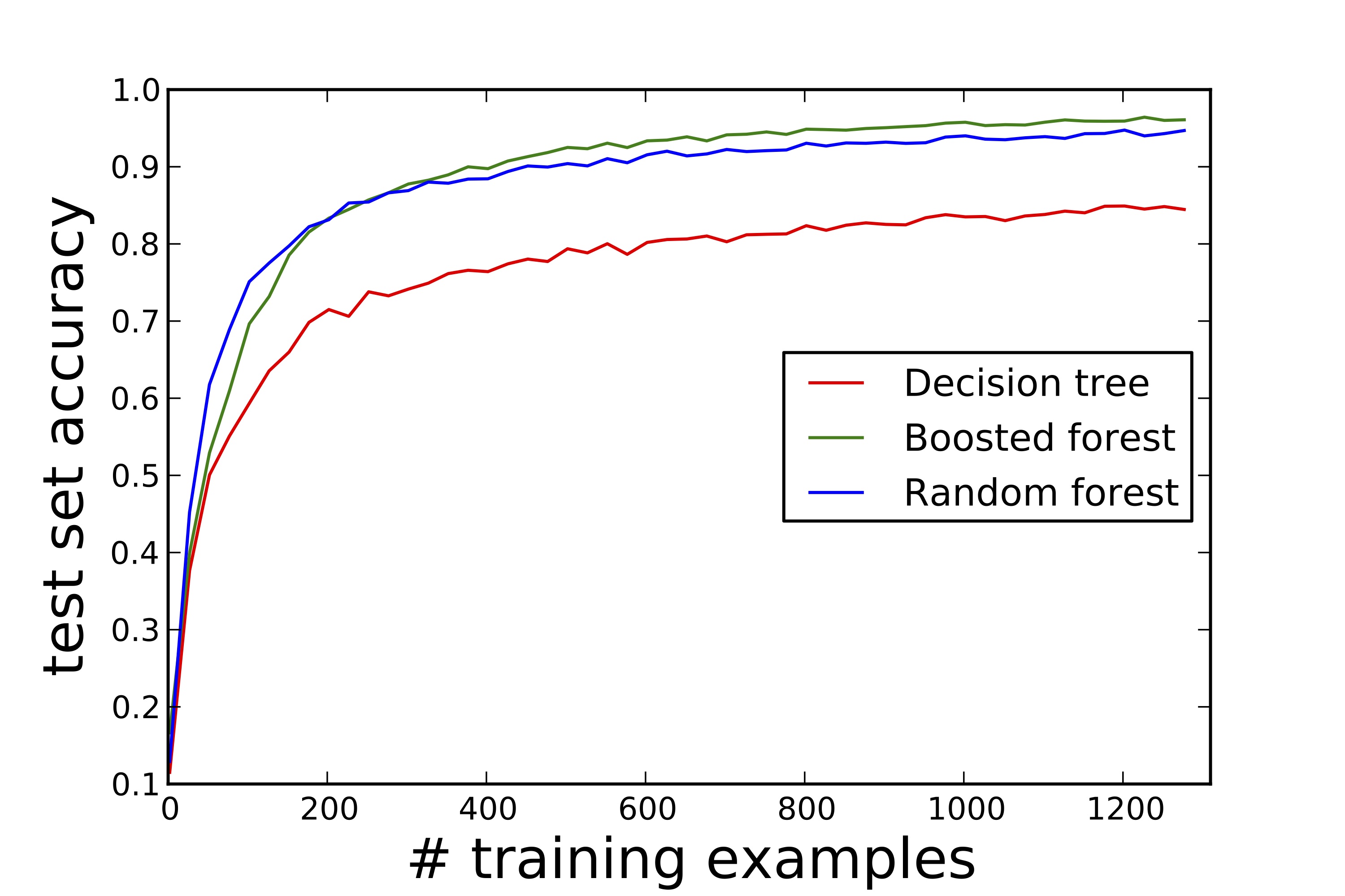
Although boosted and random forests are not as easily visualized as individual decision trees, these ensemble methods are popular because they are often quite competitive. Boosted forests typically have a slightly lower generalization error than their random forest counterparts. For this reason, they are often used when accuracy is highly-valued — see last figure for an example learning curve consistent with this rule of thumb: Generalization error rate versus training set size for a hand-written digits learning problem. However, the individual trees in a bagged forest can be constructed in parallel. This benefit — not shared by boosted forests — can favor random forests as a go-to, out-of-box approach for treating large-scale machine learning problems.
Exercises follow that detail some further points of interest relating to decision trees and their construction.
References
[1] Elements of Statistical Learning, by Hastie, Tibshirani, Friedman
[2] An Introduction to Statistical Learning, by James, Witten, Hastie, and Tibshirani
[3] Random Forests, by Breiman (Machine Learning, 45, 2001).
[4] Sk-learn documentation on runtime complexity, see section 1.8.4.
Exercises
1) Jensen’s inequality and classification tree cost functions
a) Consider a real function \(y(x)\) with non-positive curvature. Consider sampling \(y\) at values \(\{x_1, x_2, \ldots, x_m\}\). By considering graphically the centroid of the points \(\{(x_i, y(x_i))\}\), prove Jensen’s inequality,
When does equality hold?
b) Consider binary tree classification guided by the minimization of the error rate (\ref{errorrate}). If all possible cuts of a particular region always leave class \(0\) in the minority in both resulting sub-regions, will a cut here ever be made?
c) How about if (\ref{gini}) or (\ref{crossentropy}) is used as the cost function?
2) Decision tree prediction runtime complexity
Suppose one has constructed an approximately balanced decision tree, where each node contains one of the \(n\) training examples used for its construction. In general, approximately how long will it take to determine the region \(R_i\) to which a supplied feature vector belongs? How about for ensemble models? Any difference between typical bagged and boosted forests?
3) Classification tree construction runtime complexity
a) Consider a region \(R\) within a classification tree containing \(n_i\) training examples of class \(i\), with \(\sum_i n_i = N\). Now, suppose a cut is considered in which a single training example of class \(1\) is removed from the region. If the region’s cross-entropy before the cut is given by \(CE_0\), show that its entropy after the cut will be given by
If \(CE_0\), \(N\), and the \(\{n_i\}\) values are each stored in memory for a given region, this equation can be used to evaluate in \(O(1)\) time the change in its entropy with any single example removal. Similarly, the change in entropy of a region upon addition of a single training example can also be evaluated in \(O(1)\) time. Taking advantage of this is essential for obtaining an efficient tree construction algorithm.
b) Show that a region’s Gini coefficient (\ref{gini}) can also be updated in \(O(1)\) time with any single training example removal.
4)Regression tree construction runtime complexity.
Consider a region \(R\) within a regression tree containing \(N\) training examples, characterized by mean label value \(\overline{y}\) and cost value (\ref{treecost}) given by \(J\) (\( N\) times the region’s label variance). Suppose a cut is considered in which a single training example having label \(y\) is removed from the region. Show that after the cut is taken the new mean training label and cost function values within the region are given by
These results allow for the cost function of a region to be updated in \(O(1)\) time as single examples are either inserted or removed from it. Their simplicity is a special virtue of the squared error cost function. Other cost function choices will generally require significant increases in tree construction runtime complexity, as most require a fresh evaluation with each new subset of examples considered.
5) Chebychev’s inequality and random forest classifier accuracy
Adapted from [3].
a) Let \(x\) be a random variable with well-defined mean \(\mu\) and variance \(\sigma^2\). Prove Chebychev’s inequality,
b) Consider a binary classification problem aimed at fitting a sampled function \(y(\textbf{f})\) that takes values in \(\{ 0,1\}\). Suppose a decision tree \(h_{\theta}(\textbf{f})\) is constructed on the samples using a greedy, randomized approach, where the randomization is characterized by the parameter \(\theta\). Define the classifier’s margin \(m\) at \(\textbf{f}\) by
This is equal to \(1\) if \(h_{\theta}\) and \(y\) agree at \(\textbf{f}\), and \(-1\) otherwise. Now, consider a random forest, consisting of many such trees, each obtained by sampling from the same \(\theta\) distribution. Argue using (\ref{Cheby}), (\ref{tree_margin_def}), and the law of large numbers that the generalization error \(GE\) of the forest is bounded by
c) Show that
d) Writing,
for the \(\theta\), \(\theta^{\prime}\)-averaged margin-margin correlation coefficient, show that
Combining with (\ref{rf_bound}), this gives
The bound (\ref{tree_bound_final}) implies that a random forest’s generalization error is reduced if the individual trees making up the forest have a large average margin, and also if the trees are relatively-uncorrelated with each other.
Cover image by roberts87, creative commons license.
Appendix: python/sk-learn implementations
Here, we provide the python/sk-learn code used to construct the final figure in the body of this note: Learning curves on sk-learn’s “digits” dataset for a single tree, a random forest, and a boosted forest.
from sklearn.datasets import load_digits
from sklearn.tree import DecisionTreeClassifier
from sklearn.ensemble import RandomForestClassifier
from sklearn.ensemble import GradientBoostingClassifier
import numpy as np

# load data: digits.data and digits.target,
# array of features and labels, resp.
digits = load_digits(n_class =10)

n_train = []
t1_accuracy = []
t2_accuracy = []
t3_accuracy = []

# below, we average over "trials" num of fits for each sample
# size in order to estimate the average generalization error.
trials = 25

clf = DecisionTreeClassifier()
clf2 = GradientBoostingClassifier(max_depth=3)
clf3 = RandomForestClassifier()

num_test = 500

# loop over different training set sizes
for num_train in range(2,len(digits.target)-num_test,25):

acc1, acc2, acc3 = 0,0,0

for j in range(trials):
    perm = [0]
    while len(set(digits.target[perm[:num_train]]))<2:
        perm = np.random.permutation(len(digits.data))

    clf = clf.fit(
        digits.data[perm[:num_train]],
        digits.target[perm[:num_train]])
    acc1 += clf.score(
        digits.data[perm[-num_test:]],
        digits.target[perm[-num_test:]])

    clf2 = clf2.fit(
        digits.data[perm[:num_train]],
        digits.target[perm[:num_train]])
    acc2 += clf2.score(
        digits.data[perm[-num_test:]],
        digits.target[perm[-num_test:]])

    clf3 = clf3.fit(
        digits.data[perm[:num_train]],
        digits.target[perm[:num_train]])
    acc3 += clf3.score(
        digits.data[perm[-num_test:]],
        digits.target[perm[-num_test:]])

    n_train.append(num_train)
    t1_accuracy.append(acc1/trials)
    t2_accuracy.append(acc2/trials)
    t3_accuracy.append(acc3/trials)

%pylab inline
plt.plot(n_train,t1_accuracy, color = 'red')
plt.plot(n_train,t2_accuracy, color = 'green')
plt.plot(n_train,t3_accuracy, color = 'blue')
 Jonathan grew up in the midwest and then went to school at Caltech and UCLA. Following this, he did two postdocs, one at UCSB and one at UC Berkeley. His academic research focused primarily on applications of statistical mechanics, but his professional passion has always been in the mastering, development, and practical application of slick math methods/tools. He currently works as a data-scientist at Stitch Fix.