We review the two essentials of principal component analysis (“PCA”): 1) The principal components of a set of data points are the eigenvectors of the correlation matrix of these points in feature space. 2) Projecting the data onto the subspace spanned by the first \(k\) of these — listed in descending eigenvalue order — provides the best possible \(k\)-dimensional approximation to the data, in the sense of captured variance.
Introduction
One way to introduce principal component analysis is to consider the problem of least-squares fits: Consider, for example, the figure shown below. To fit a line to this data, one might attempt to minimize the squared \(y\) residuals (actual minus fit \(y\) values). However, if the \(x\) and \(y\) values are considered to be on an equal footing, this \(y\)-centric approach is not quite appropriate. A natural alternative is to attempt instead to find the line that minimizes the total squared projection error: If \((x_i, y_i)\) is a data point, and \((\hat{x}_i, \hat{y}_i)\) is the point closest to it on the regression line (aka, its “projection” onto the line), we attempt to minimize
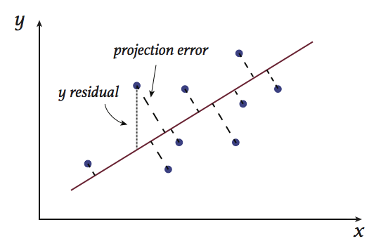
The summands here are illustrated in the figure: The dotted lines shown are the projection errors for each data point relative to the red line. The minimizer of (\ref{score}) is the line that minimizes the sum of the squares of these values.
Generalizing the above problem, one could ask which \(k\)-dimensional hyperplane passes closest to a set of data points in \(N\)-dimensions. Being able to identify the solution to this problem can be very helpful when \(N \gg 1\). The reason is that in high-dimensional, applied problems, many features are often highly-correlated. When this occurs, projection of the data onto a \(k\)-dimensional subspace can often result in a great reduction in memory usage (one moves from needing to store \(N\) values for each data point to \(k\)) with minimal loss of information (if the points are all near the plane, replacing them by their projections causes little distortion). Projection onto subspaces can also be very helpful for visualization: For example, plots of \(N\)-dimensional data projected onto a best two-dimensional subspace can allow one to get a feel for a dataset’s shape.
At first glance, the task of actually minimizing (\ref{score}) may appear daunting. However, it turns out this can be done easily using linear algebra. One need only carry out the following three steps:
- Preprocessing: If appropriate, shift features and normalize so that they all have mean \(\mu = 0\) and variance \(\sigma^2 = 1\). The latter, scaling step is needed to account for differences in units, which may cause variations along one component to look artificially large or small relative to those along other components (eg, one raw component might be a measure in centimeters, and another in kilometers).
- Compute the covariance matrix. Assuming there are \(m\) data points, the \(i\), \(j\) component of this matrix is given by:
$$\tag{2} \label{2} \Sigma_{ij}^2 = \frac{1}{m}\sum_{l=1}^m \langle (f_{l,i} - \mu_i) (f_{l,j} - \mu_j) \rangle\\ = \langle x_i \vert \left (\frac{1}{m} \sum_{l=1}^m \vert \delta f_l \rangle \langle \delta f_l \vert \right) \vert x_j \rangle.$$Note that, at right, we are using bracket notation for vectors. We make further use of this below — see footnote [1] at bottom for review. We’ve also written \(\vert \delta f_l \rangle\) for the vector \(\vert f_l \rangle - \sum_{i = 1}^n \mu_i \vert x_i \rangle\) — the vector \(\vert f_l \rangle\) with the dataset’s centroid subtracted out.
- Project all feature vectors onto the \(k\) eigenvectors \(\{\vert v_j \rangle\), \(j = 1 ,2 \ldots, k\}\) of \(\Sigma^2\) that have the largest eigenvalues \(\lambda_j\), writing
$$\tag{3} \label{3} \vert \delta f_i \rangle \approx \sum_{j = 1}^k \langle v_j \vert \delta f_i \rangle \times \vert v_j\rangle. $$The term \(\langle v_j \vert \delta f_i \rangle\) above is the coefficient of the vector \(\vert \delta f_i \rangle\) along the \(j\)-th principal component. If we set \(k = N\) above, (\ref{3}) becomes an identity. However, when \(k < N\), the expression represents an approximation only, with the vector \(\vert \delta f_i \rangle\) approximated by its projection into the subspace spanned by the largest \(k\) principal components.
The steps above are all that are needed to carry out a PCA analysis/compression of any dataset. We show in the next section why this solution will indeed provide the \(k\)-dimensional hyperplane resulting in minimal dataset projection error.
Mathematics of PCA
To understand PCA, we proceed in three steps.
- Significance of a partial trace: Let \(\{\textbf{u}_j \}\) be some arbitrary orthonormal basis set that spans our full \(N\)-dimensional space, and consider the sum
\begin{align}\tag{4} \label{4} \sum_{j = 1}^k \Sigma^2_{jj} = \frac{1}{m} \sum_{i,j} \langle u_j \vert \delta f_i \rangle \langle \delta f_i \vert u_j \rangle\\ = \frac{1}{m} \sum_{i,j} \langle \delta f_i \vert u_j \rangle \langle u_j \vert \delta f_i \rangle\\ \equiv \frac{1}{m} \sum_{i} \langle \delta f_i \vert P \vert \delta f_i \rangle. \end{align}To obtain the first equality here, we have used \(\Sigma^2 = \frac{1}{m} \sum_{i} \vert \delta f_i \rangle \langle \delta f_i \vert\), which follows from (\ref{2}). To obtain the last, we have written \(P\) for the projection operator onto the space spanned by the first \(k\) \(\{\textbf{u}_j \}\). Note that this last equality implies that the partial trace is equal to the average squared length of the projected feature vectors — that is, the variance of the projected data set.
- Notice that the projection error is simply given by the total trace of \(\Sigma^2\), minus the partial trace above. Thus, minimization of the projection error is equivalent to maximization of the projected variance, (\ref{4}).
- We now consider which basis maximizes (\ref{4}). To do that, we decompose the \(\{\textbf{u}_i \}\) in terms of the eigenvectors \(\{\textbf{v}_j\}\) of \(\Sigma^2\), writing
\begin{align} \tag{5} \label{5} \vert u_i \rangle = \sum_j \vert v_j \rangle \langle v_j \vert u_i \rangle \equiv \sum_j u_{ij} \vert v_j \rangle. \end{align}Here, we’ve inserted the identity in the \(\{v_j\}\) basis, and written \( \langle v_j \vert u_i \rangle \equiv u_{ij}\). With these definitions, the partial trace becomes\begin{align}\tag{6} \label{6} \sum_{i=1}^k \langle u_i \vert \Sigma^2 \vert u_i \rangle = \sum_{i,j,l} u_{ij}u_{il} \langle v_j \vert \Sigma^2 \vert v_l \rangle \\= \sum_{i=1}^k\sum_{j} u_{ij}^2 \lambda_j. \end{align}The last equality here follows from the fact that the \(\{\textbf{v}_i\}\) are the eigenvectors of \(\Sigma^2\) — we have also used the fact that they are orthonormal, which follows from the fact that \(\Sigma^2\) is a real, symmetric matrix. The sum (\ref{6}) is proportional to a weighted average of the eigenvalues of \(\Sigma^2\). We have a total mass of \(k\) to spread out amongst the \(N\) eigenvalues. The maximum mass that can sit on any one eigenvalue is one. This follows since \(\sum_{i = 1}^k u_{ij}^2 \leq \sum_{i = 1}^N u_{ij}^2 =1\), the latter equality following from the fact that \( \sum_{i = 1}^N u_{ij}^2\) is an expression for the squared length of \(\vert v_j\rangle\) in the \(\{u_i\}\) basis. Under these constraints, the maximum possible average one can get in (\ref{6}) occurs when all the mass sits on the largest \(k\) eigenvalues, with each of these eigenvalues weighted with mass one. This condition occurs if and only if the first \(k\) \(\{\textbf{u}_i\}\) span the same space as that spanned by the first \(k\) \(\{\textbf{v}_j\}\) — those with the \(k\) largest eigenvalues.
That’s it for the mathematics of PCA.
Footnotes
[1] Review of bracket notation: \(\vert x \rangle\) represents a regular vector, \(\langle x \vert\) is its transpose, and \(\langle y \vert x \rangle\) represents the dot product of \(x\) and \(y\). So, for example, when the term in parentheses at the right side of (\ref{2}) acts on the vector \(\vert x_j \rangle\) to its right, you get \( \frac{1}{m} \sum_{k=1}^m \vert \delta f_k \rangle \left (\langle \delta f_k \vert x_j \rangle\right).\) Here, \( \left (\langle \delta f_k \vert x_j \rangle\right)\) is a dot product, a scalar, and \(\vert \delta f_k \rangle\) is a vector. The result is thus a weighted sum of vectors. In other words, the bracketed term (\ref{2}) acts on a vector and returns a linear combination of other vectors. That means it is a matrix, as is any other object of form \(\sum_i \vert a_i \rangle \langle b_i \vert\). A special, important example is the identity matrix: Given any complete, orthonormal set of vectors \(\{x_j\}\), the identity matrix \(I\) can be written as \(I = \sum_i \vert x_i \rangle \langle x_i \vert\). This identity is often used to make a change of basis.
 Jonathan grew up in the midwest and then went to school at Caltech and UCLA. Following this, he did two postdocs, one at UCSB and one at UC Berkeley. His academic research focused primarily on applications of statistical mechanics, but his professional passion has always been in the mastering, development, and practical application of slick math methods/tools. He currently works as a data-scientist at Stitch Fix.