With an eye towards predicting traffic evolution, we begin by examining the time-dependence of the contribution from the first principal components on different days of the week. Traffic throughout the day \(\vert x(t) \rangle\) can be represented in the basis of principal components; \(\vert x(t) \rangle = \sum_{i} c_i(t) \vert \phi_i \rangle \)\(^1\), where \(\vert \phi_i \rangle\) is the ith principle component. The coefficients \(c_i(t)\), sometimes called the “scores” of \(\vert x(t) \rangle\) in the basis of principal components, carry all of the dynamics.
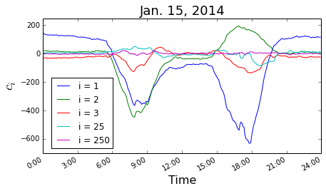
The largest deviations in the traffic patterns (and of the scores) are during weekday rush hours (around 8 am and 5 pm) - see plot of the scores for several modes throughout Jan. 15. There is an abundance of interesting information to be gleaned here. First, note that, generally, the amplitude of the lowest modes is the largest, again, as expected. In addition, there appears to be some large wavelength structure (primarily correlated with the rush hours) sitting on top of a background of higher frequency noise. Ignoring for the moment the noise, the modes generally come in two classes - something like “even” and “odd”. That is, some fluctuate with the same sign in both the morning and evening, while others fluctuate with opposite signs.
Let us consider the first two modes in this plot. The first mode is an even mode and we attribute this essentially to an overall shift in general speed throughout the system. Whenever there are more cars on the road, the speed generally decreases everywhere. Indeed, this is the only mode that deviates significantly from zero at night and it deviates positive - the roads are generally completely clear at night and thus the speed is somewhat higher than average. The second mode is an odd mode, which we attribute generally to directional traffic - when everyone is going to work it has one sign, when they are coming home it has the other. We have previously visualized these two modes and, indeed, these concepts are reflected in their spatial structure: the first mode is generally uniform while the second has regions with either sign and many sections of highway are positive in one direction and negative in the other.
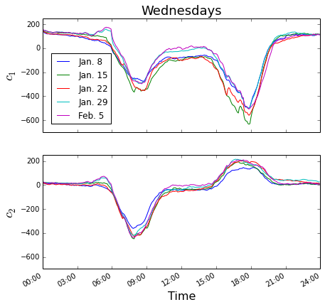
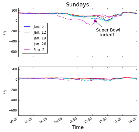
The time-dependence of these scores is remarkably consistent from week to week (See Wednesdays plot below of the scores for modes 1 and 2). On the right, we plot the same quantities for several Sundays as well. Not surprisingly, the fluctuations are smaller on Sundays than on weekdays, reflecting more homogeneous speeds in sparse traffic. However, they are still reproducible from week to week - see Sundays Jan. 5, 12, 19, and 26 - apparently there is a slight slow-down around 6 pm. Feb. 2 was Super Bowl Sunday and the traffic pattern differs qualitatively from other Sundays. Remarkably, we can identify the time of the Super Bowl kickoff from this data - before the kickoff there is slightly more traffic than the average Sunday and immediately after, less.
[1] On projecting into principal components: In the original basis, our data reads \(\vert x(t) \rangle = \sum_j a_j(t) \vert \ell_j \rangle\), where the sum runs over all loop locations(there are some 2,000 loops in the Bay area) and \(\vert \ell_j \rangle\) is a unit fluctuation in speed at the location of loop \(j\). Changing bases, to the principal components \(\vert \phi_i \rangle\), \(\vert x(t) \rangle = \sum_{i,j} a_j(t) \vert \phi_i \rangle \langle \phi_i \vert \ell_j \rangle\) \(= \sum_i c_i(t) \vert \phi_i \rangle\) where \(c_i(t) = \sum_j a_j(t) \langle \phi_i \vert \ell_j \rangle\). The coefficient \(\langle \phi_i \vert \ell_j \rangle\) is often called the “loading” of \(\vert \ell_j \rangle\) into \(\vert \phi_i \rangle\).
 Dustin got a B.S in Engineering Physics from the Colorado School of Mines (Golden, CO) before moving to UC Santa Barbara for graduate school. There he became interested in Soft Condensed Matter Physics and Polymer Physics, studying the interaction between single DNA molecules and salt ions. After a brief postdoc at UC San Diego studying the physics of bacterial growth, Dustin decided to move into the data science business for good - he is now a Quantitative Analyst at Google in Mountain View.